Some time ago, I wrote an article about upgrading code from .NET Framework to .NET Core. While this may give you a decent overview to get your code up and running in .NET Core, the devil is, as always, in the details. So let me give you an example of such a detail.
In this case, getting your code up and running in .NET Core is one thing. But in the case of user interfaces, more specifically when they are using WinForms, there’s a difference between having them up and running, and having them look and behave correctly.
Namely, when you design forms with the Designer in Visual Studio, a lot of code is generated automatically, and you may not have given it any second thought. But one thing that is relevant, is that the Designer will generate components that have the AutoScaleMode property set to Font.
What does that mean exactly? Well, it may seem a bit unusual to scale things by a ‘font’, but the idea is that your controls will not have an absolute size, but will scale depending on the size of the system’s fonts. Which makes sense when you mostly want to display readable text, and are not worried about absolute size.
So, what this means is that it is likely that when you’ve designed a number of forms/controls with the Visual Studio Designer, that they will have font-relative scaling. So far so good, but what’s the problem then?
Well, the question is: WHAT font is being used for scaling? That is the Font property of the control. Which you probably, just like the AutoScaleMode properly, rarely set manually. In which case, it will default to the DefaultFont.
Well, there’s our small print: For .NET Core 3 there was a breaking change: the default font was changed from Microsoft Sans Serif 8 to Segoe UI 9. That explains why the default behaviour differs between .NET Framework and .NET Core 3.1 or higher. The scaling is based off a different font. The differences are generally subtle, so you may not even notice in most screens. But sometimes things will look very wrong.
However, we’re in luck. Because .NET 6 introduced another change, which can help us here: A new Application.SetDefaultFont() function was added, which allows you to set the default font application-wide at startup. If you set it to Microsoft Sans Serif 8 at startup, the font-relative scaling in your application will behave the same as it did .NET Framework. That means you won’t have to manually set the font for every control.
However, the tricky thing here is that this behaviour was changed in .NET Core 3, a very early version, from the days when .NET Core was not yet considered ready for mainstream/desktop usage. As I wrote last time, that wasn’t until .NET 5. But as we now see, it may be useful to read through the entire changelog of .NET Core whenever we run into an issue, even the early versions, as some breaking changes may have been done early on, and they may affect us now.
The other day I read this in-depth article on font usage in early DOS games by VileR. Since some of the fonts were apparently stored not as 1-bit bitmaps, but as multiple bits per pixel, I was wondering when the usage of multicolour fonts became commonplace on the PC.
I randomly thought of Lemmings as a game that I recall using a very nice and detailed font. But that turned out to be quite the can of worms, so I thought I’d write a quick summary of what we uncovered.
Now Lemmings was a game originally developed on the Amiga, and then ported to many different platforms. I mostly played the Amiga game back in the day, although I did also have a copy of the PC version. I had a vague recollection that although the Amiga version did look somewhat better, the PC version used basically the same font as the Amiga version.
Let’s compare the Amiga and PC version of Lemmings. And while we’re at it, let’s throw in the Atari ST version as well. More specifically, let’s concentrate on the VGA version of Lemmings for PC. Then we have three machines that have roughly similar video capabilities. All three machines have a video mode of 320×200, and support a palette that can be user-defined by RGB values. The Atari ST supports 3 bits per component (512 colours in total), the Amiga supports 4 bits per component (4096 colours in total), and VGA supports 6 bits per component (262144 colours in total).
The Atari ST supports 16 colours at once, the Amiga supports 32 colours at once (or 64 colours in the special ‘Extra HalfBrite’ mode), and VGA supports 256 colours at once. So at first glance, all three machines appear to have similar capabilities, with the Atari ST being the most limited, and VGA being the most capable. But now let’s look at how the game looks on these three systems.
First, the original on the Amiga:
Then the Atari ST:
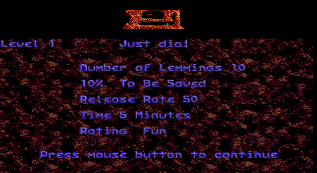
Okay, looks very similar at first glance, although there is something I couldn’t quite put my finger on at first glance. But let’s look at the VGA version first:
Hum, wait a second… When I look for screenshots on the internet, I also find some that look like this:
Are there different versions of Lemmings for PC? Well, yes and no, as it turns out. When you start the game, there is a menu that asks what machine type you have:
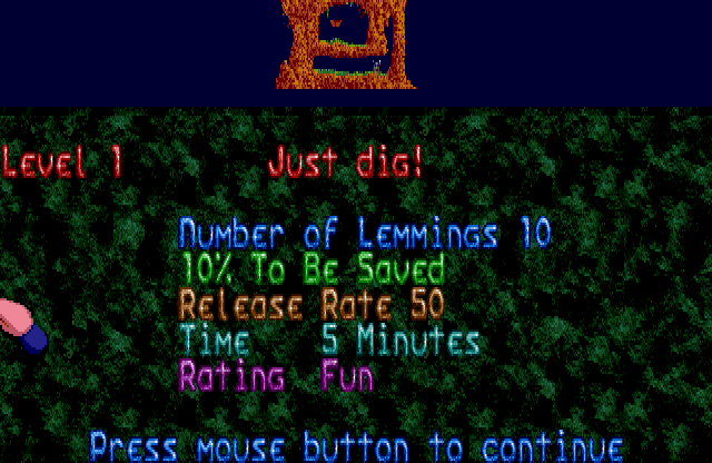
The first screenshot is from the game in “For PC compatibles” mode, the second screenshot is “For High Performance PCs”. So let’s call the first ‘lo’ mode, and the second ‘hi’ mode.
Okay, so let’s inspect things closer here. At first glance, the main level view appears to be the same on all three systems. That would imply that only 16 colours are used on all systems, otherwise the Atari ST would not be able to keep up visually with the others.
The only difference that stands out is that the Amiga and Atari ST have a blue-ish background colour, where the VGA versions are black. It’s not entirely clear why that is. Also, the blue background is used only for the level on Amiga, where the background is black for the text and icons. On the Atari ST, the background for the text is blue, and it only switches to black for the icons.
But then we get to the part that kicked this off in the first place: the font. On the Amiga we see a very detailed font, using various shades of green. On the Atari ST, we see a font that looks the same, at first glance (more on that later). On the ‘lo’ VGA version, we see a font with the same basic shape, but it appears to only have two shades: one green and one white.
The ‘hi’ VGA version however, looks different. For some reason, the font is not as high. Instead of the font filling out the entire area between the level view and the icon bar, there are 4 black scanlines between the level and the font. The icons are the same size and in the same position on screen, so effectively the font is scaled down a bit. It is only 11 pixels high, where the others are 15 pixels high. The font has more shades of green here: a number of 4 in total. Still less than on the Amiga (I count 7 shades there) and Atari ST (5 shades).
Okay, so there is something going on here. But what exactly? Well, we are being tricked! The game runs in a 16-colour mode on all three systems. However, if you inspect the screenshots closely, you will see that there are actually more than 16 colours on screen. As already mentioned, the font itself uses various shades of green. You don’t see that many shades of green in the level. That implies that the palette is changed between the level and the font.
This explains why the PC version has a ‘lo’ and a ‘hi’ version: Because VGA is not synchronized to the system clock, it is not trivial to change the palette at a given place on screen. While it is possible (see also my 1991 Donut), it will require some clever timer interrupts and recalibrating per-frame to avoid drift. So that explains why they chose to only do this on high performance PCs. On a slow PC, it would slow down the game too much. It also explains why there are 4 black scanlines between the level and the font. Firstly, because of all the different PCs out there, it is very hard to predict exactly how long the palette change takes. So you’ll want a bit of margin to avoid visible artifacts. Secondly, various VGA implementations won’t allow the RAMDAC to read the palette registers while the CPU is updating them. This can lead to black output or artifacts similar to CGA snow. But if all pixels are black, you won’t notice.
So apparently the ‘hi’ version does perform a palette change, where the ‘lo’ version does not. That means the ‘lo’ version can only use colours that are already in the level palette for its font. It also explains why the icons don’t have the brownish colours of the other three versions: the icons also have to make do with whatever is in the palette.
But getting back to the ‘hi’ version… Its icons still don’t look as good as the Amiga and Atari ST versions. We can derive why this is: we do not see any black scanlines between the font and icons. So we know that the ‘hi’ version does not perform a second palette change between font and icons. The Amiga and Atari ST versions do, however. On the PC, this wouldn’t have been practical. They would have had to sacrifice another few black scanlines, and the CPU requirements would have gone up even further. So apparently this was the compromise. That means that a single 16-colour palette is shared between the font and the icons.
Speaking of which, during the in-between screens, the VGA version also changes palette:
The top part shows the level in 16 colours. Then there are a few black scanlines, where the palette is changed to the brown earth colours and the blue shades for the font.
Mind you, that is still a simplification of how it looks on the Amiga:
Apparently the Amiga version changes the palette at every line of text. The PC is once again limited to changing the palette once, in an area with a few black scanlines. In this case, both the ‘lo’ and ‘hi’ versions appear to do the same. Performance was not an issue with a static info screen, apparently.
The Amiga uses 640×200 resolution here. The PC instead uses 640×350. That explains why the PC version has a somewhat strange aspect ratio for the level overview.
But getting back to the font and icons in-game. They do look a bit more detailed on the Amiga than on the Atari ST. And it’s not just the colours, it seems. So what is going on here? Well, possibly the most obvious place to spot it is the level overview in the bottom-right corner. Yes, it has twice the horizontal resolution of the other platforms. Apparently it is running in 640×200 resolution, rather than 320×200.
That explains why the icons look slightly different as well. They are a more detailed high-resolution version than the other platforms. And if we look closer at the font, we see that this is the high-resolution font that is also used in the other screen.
The Atari ST cannot do this, because it does not have a 640×200 mode that is capable of 16 colours. And for VGA, as already said, it’s not possible to accurately perform operations at a given screen position. So if you can’t accurately change palettes, you certainly can’t accurately change display resolution.
So there we have it, three systems with very similar graphics capabilities on paper, yet we find that there are 4 different ways in which the game Lemmings is actually rendered. Clever developers pushing the limits of each specific system.
I suppose the biggest unanswered question is: why does the VGA version have this limitation? Worst-case, you have 3 palettes of 16 colours on screen, which is 48 colours. In mode 13h, you can have 256 colours, so no palette changes would be required. Instead the developers appear to have chosen to use the same 16-colour mode for both EGA and VGA, and only improve the palette for the VGA version. This may be because they use EGA functionality for scrolling and storing sprites offscreen. In mode 13h you wouldn’t have that. You’d have to perform scrolling by copying data around in memory. That may have been too slow. And perhaps they weren’t familiar with mode X. Or perhaps they tried mode X, but found that it was too limiting, so they stuck with EGA mode 0Dh anyway. Or perhaps they figured they’d need separate content for a mode X mode, which would require too much extra diskspace. Who knows.
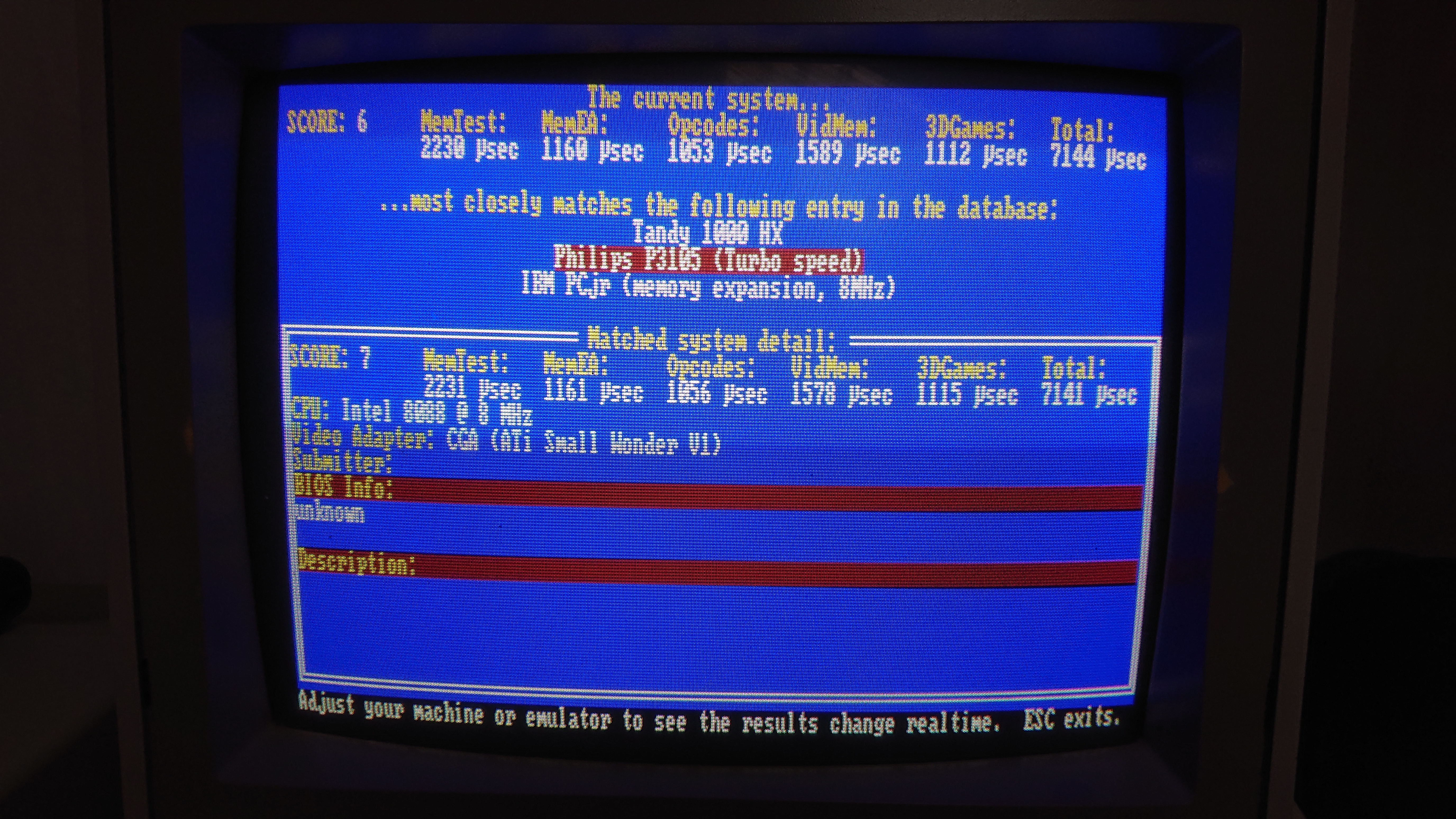
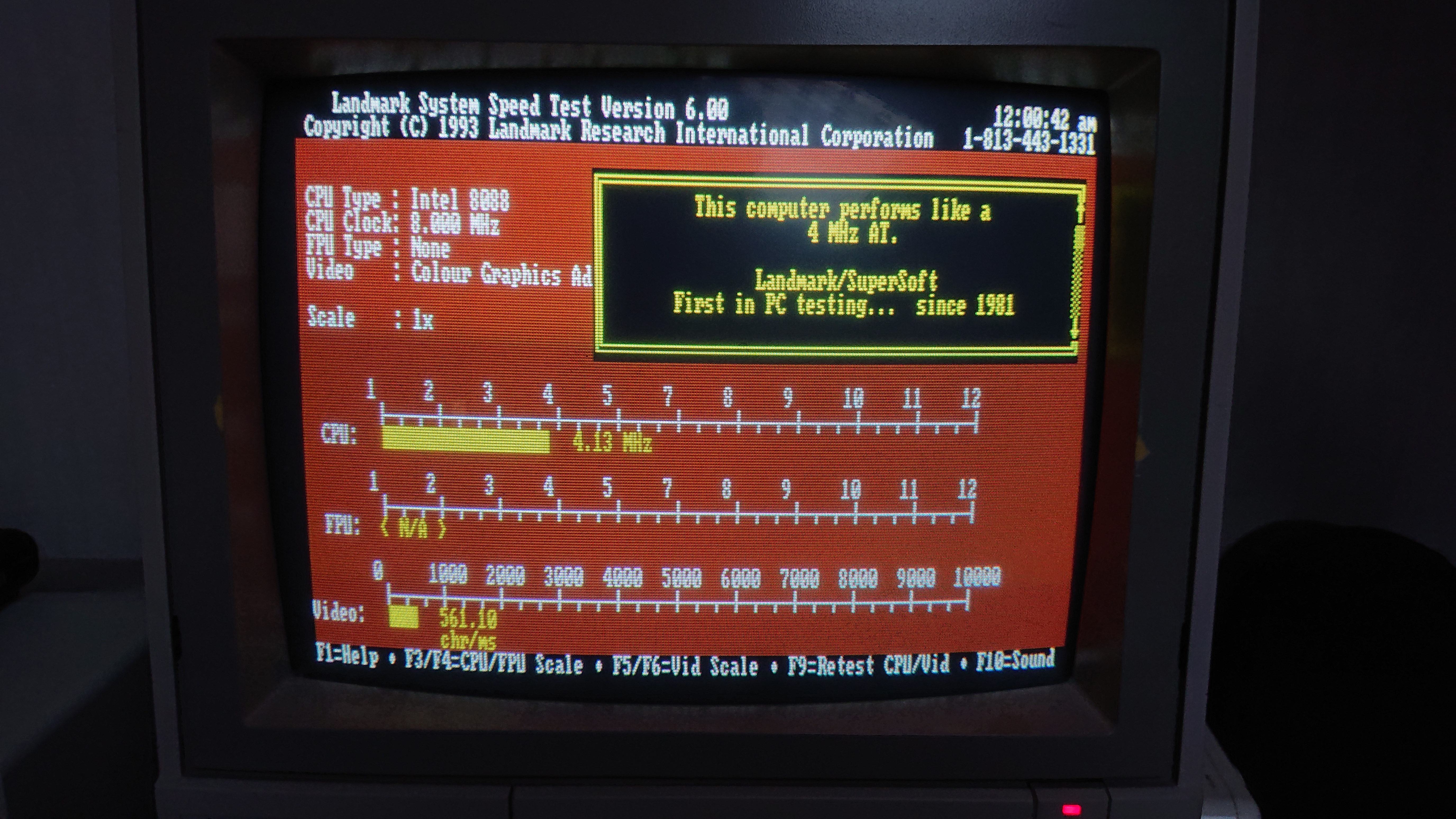
For my modifications to the XDC player, I targeted my Philips 3105 XT clone. It has a turbo mode of 8 MHz, and an ATi Small Wonder CGA clone. The harddisk is a 32MB Disk-on-Module connected to an XT-IDE card.
8 MHz you say? Yes, I was somewhat surprised by that myself. Most turbo XT machines will derive their clockspeed from the NTSC base clock of 14.31818. So common speeds are 4.77 MHz, 7.16 MHz and 9.54 MHz.
So I checked with TOPBench and Landmark, and they both confirmed that this CPU is actually running at 8 MHz:
I wrote a simple tool that can halve the sample rate of the audio in a video file, and also preprocess the audio to PWM or Tandy formats, so there is no translation required at runtime, reducing CPU overhead.
The first attempt wasn’t too successful… The machine wasn’t quite fast enough. Or, the code wasn’t quite fast enough, depending on how you look at it. This resulted in a few buffer underruns, causing the PC speaker to glitch, as it would play garbage data at this point (it also does this at the start of each video, as there is no data buffered yet). So I performed some optimization in assembly, and some other minor performance tweaks, and after a few tries, I came up with a version that can *almost* play the 8088 Domination content with 11 kHz PC speaker audio:
As you can see, there is still one place in the video where there’s an underrun, but it quickly solves itself, and it continues playing (with audio and video in sync of course). I suppose that is close enough for me. If I were to optimize the code further, I don’t think I could do it with the inline assembler in Pascal. Besides, the performance is highly dependent on all the hardware. With just a slightly faster video card or a slightly faster HDD controller, this machine could probably play it without a glitch. And the more common 9.54 MHz turbo XTs should also have no problem with it. Nor would a 6 MHz AT.
Oh, and yes, the Bad Apple part is missing. That’s because my HDD is only 32 MB, so I can’t fit all videos on the disk at the same time.
If you want to try this modified version of 8088 Domination for yourself, you can download it here.
Playing video on MS-DOS… it kinda was a thing with things such as the GRASP/GLPro and FLIC formats back in the day. But not on REALLY low-end machines, such as 8088s and CGA. Until the demo 8088 Corruption was released in 2004. And then its successor 8088 Domination in 2014, which I already discussed earlier.
It can play videos at very acceptable quality on an 8088 at 4.77 MHz with (composite) CGA and a Sound Blaster 2.0.
Wait, a Sound Blaster 2.0? That is a bit of an anachronism, is it not? Yes, but for two good reasons:
The Sound Blaster was the first commonly available sound solution for the IBM PC that could take advantage of the DMA controller for sample playback, thereby reducing CPU load to near-zero.
As discussed here earlier, the early Sound Blasters had some shortcomings that meant they weren’t capable of seamless playback. The 2.0 version was the first to solve this (this was fixed by implementing new commands in the firmware of the DSP. Creative also sold upgrades for SB 1.x cards to get the new 2.0 firmware, solving this issue).
Okay, so the Sound Blaster 2.0 was the first *good* solution for digital audio playback. But, one may argue… An IBM PC with a 4.77 MHz 8088 and CGA is not in the ‘good’ category either, is it? The point is “let’s see what we can do anyway”. What if we also apply this to audio?
I’ve had this idea for a while. Since I had done a streaming audio solution on PC speaker on my IBM 5160 PC/XT, I wanted to add video as well. It would make sense to combine the two, as I already wrote at the time. And the past few days I had a bit of spare time, so I decided give it a quick-and-dirty try.
As you can see from the commits, I added my code for auto-EOI to shave off a few cycles with each interrupt. For the Sound Blaster and ‘quiet’ options, this is not required, because there is only one interrupt per frame. But for the PC speaker and various other sound sources that don’t support DMA, you need an interrupt for every individual sample, so I enable auto-EOI in those cases.
I then added some PC speaker routines to enable PWM playback. I use a simple translation table that translates the unsigned 8-bit PCM samples in the XDV file to the correct PWM values. Note that the PWM values are dependent on the sample rate, so the table is initialized at runtime, when the sample rate of the file is known.
And that pretty much took care of things already. PC speaker sound is now working. There is extra CPU overhead of course, so you’ll either need a faster machine to play the same content, or you need to encode your content with a lower sample rate, and perhaps also reduce the frame rate and/or the MAXDISKRATE value when encoding. I would not recommend PC speaker on a 4.77 MHz machine at all, but on a turbo XT at 8 or 10 MHz, you should be able to get away with it reasonably well, as long as you keep the sample rate low enough, say between 8 and 11 kHz. It will be a bit of trial-and-error to find what works best for your specific machine.
Then Covox…
Now that I had a solution that could bit-bang samples, I figured I might as well add some other common devices. One is the Covox, which was trivial, as the 8-bit unsigned PCM samples could be sent to the Covox as-is. This makes it slightly faster than the PC speaker solution. It also sounds better. The quality is almost as good as the Sound Blaster. The main issue is that the interrupt-driven sample playback is more susceptible to jitter than DMA transfers are. On a fast enough machine that won’t be an issue, but on 8088s you may hear some minor jitter.
And Tandy…
Tandy is another interesting target. XDC already supports Tandy video modes, so adding Tandy audio would make sense. It can do PC speaker playback of course, but PWM also gives an annoying carrier wave. Sample playback on the SN76496 chip does not have that issue. You can get 4-bit PCM from the sound chip’s volume register. The volume is non-linear however, so you can’t just take the high nibble from the 8-bit source samples (it works, but it’s suboptimal). Instead you should use a translation table from the linear 8-bit samples to the correct non-linear 4-bit volume settings. That’s simple enough. I could just use the same approach as for the PC speaker, but with a different table.
The Tandy threw me a bit of a curveball though. I had done PCjr sample playback before, so I thought I could just take that code as a starting point. But it gave me a weird low base note, and very loud at that. Strange, that wasn’t there before?
Where the PCjr uses an actual Texas Instruments SN76496 chip, Tandy opted for a clone instead: an NCR 8496. No big deal, you may think. But there’s a catch: for sample playback you set the SN76496 to a period value of 0. This is an undocumented feature that results in an output of 0 Hz, so effectively the output is constantly high. You can modulate it with the volume register, and presto: we have a 4-bit DAC.
The NCR 8496 however, didn’t get that memo. When you write a period of 0 to it, it interprets it as a value of 400h instead, which is one higher than the maximum period value of 3FFh you can normally set (which is very similar to the various 6845-implementations that interpret a hsync width of 0 differently). So this results in a tone of (base frequency)/1024, instead of 0 Hz. That explains the loud base note I was hearing.
But wait, sample playback works on Tandy, doesn’t it? Didn’t Rob Hubbard use a sample channel in some of that excellent music he made for Tandy games? Well yes:
So how does that work then? I decided to study the code and see what it did exactly. And indeed, I found that it set a period of 1 instead of a period of 0. On the NCR 8496 this results in the highest possible frequency it can play, rather than the lowest possible frequency that you got with a period of 0. Since this frequency is well beyond the audible spectrum (over 100 kHz), you won’t actually hear it. But you can hear the modulation with the volume register, giving you the same DAC-like effect (this same trick is also used on the SAA1099 sound chip by the way, found on the CMS/GameBlaster, for example in the game BattleTech: The Crescent Hawk’s Revenge).
So once I figured out how the NCR 8496 and SN76496 are different, it was an easy enough fix. Apparently all my code was correct after all, I should just have set a period of 1 instead of a period of 0.
Sound Blaster..
Sound Baster? That was already supported, wasn’t it? Well yes, the 2.0 version. But as I discussed earlier, you can implement streaming playback on earlier Sound Blasters as well. It will not be entirely glitch-free, but you can get acceptable results.
In this case I just went for a quick-and-dirty approach. The thing is that the audio buffer size is directly related to the frame rate. That is, an audio buffer has the exact length of one frame. That is what makes the magic work in the original XDC player: the SB will generate an interrupt when the audio buffer has completed. The interrupt handler will then display a new frame. This means that the audio buffers are extremely short.
As I said earlier, that is suboptimal, because you get a glitch everytime you start a new buffer. So ideally you want the largest possible buffers, to reduce glitching to a minimum. However, for now I just went for a quick-and-dirty solution that just restarts the audio buffer at every interrupt. It was trivial to add this to the existing code. It will result in a glitch at every frame. However, this glitching is because of the time it takes to start a new buffer on the DSP. When I wrote the article, the assumption was that you use high sample rates. As I wrote in the article, sending a new command to the DSP took about 316 CPU cycles on an 8088 at 4.77 MHz, while a single sample at 22 kHz took 216 CPU cycles. Clearly, at lower sample rates, each sample takes longer, while the DSP time should remain constant. So that means the glitches become less obvious at lower rates, and perhaps won’t be noticeable at all, given a low enough rate.
I may revisit this code at some point, and modify the buffering of audio in a way that I can apply some of the ideas in my earlier article, by using a large DMA buffer. But for now at least SB 1.x works. And the code checks the DSP version, so it only uses this fallback when a 1.x SB is detected. SB 2.0 and higher should still work as they always did, so they are not compromised in any way by this addition.
So now what?
Well, one way to use this is to create new content, targeted specifically at lower sample rates that work better on these newly supported sound devices.
Another way is to run existing content on faster machines. 8088 Domination uses 22 kHz audio, which is a pretty bad case for bit-banged devices. But a reasonably fast 286 will have no problem with that. So you should be able to play back the 8088 Domination content as-is on a fast enough machine.
A third method is to downgrade the existing content. The audio buffers are stored at the end of each frame. It is trivial to downsample the buffers in-place. A turbo XT should be able to play the video content on PC speaker/Covox when the audio is downsampled from 22 kHz to something in the range of 8-11 kHz I would think.
And when you modify the audio anyway, you could also pre-apply the translation table, so it won’t have to be done at runtime, shaving off some precious CPU-cycles per sample, which will definitely improve performance. Some extra feature flags could be introduced to the feature-byte of the XDV-format to mark PWM-encoded or Tandy-encoded audio.
Anyway, feel free to experiment and have fun. See the next post for some of my results, and a modified version of 8088 Domination to toy around with.
Say there’s a person who makes some weird claims about the Amiga graphics system, like saying the Amiga doesn’t have any ‘400-line modes’, and it’s only low quality TV-resolution…
Another person then says the Amiga in fact does have a 480-line mode in NTSC and a 512-line mode in PAL, it’s just that they are interlaced, to be compatible with NTSC/PAL standard equipment, but they can be deinterlaced and promoted to 31 kHz signals using a device known as a ‘flicker fixer‘.
Then this person also points out that the IBM PC also started out based on NTSC signals, given that the CGA card was designed to output NTSC-compatible composite signal, and also has a header for an RF-modulator to connect it to a TV.
Now, these are facts that should be easy to verify, one would think. The Amiga specs are well-known, and it may not be THAT well-known that CGA has an RF header, but it is documented in the CGA manual, and early IBM PC ads also specifically mention that the PC “hooks up to your home TV”.
So you’d think that the first person would accept these facts as facts. But instead, this person starts making personal attacks at the other person, and denies these facts, simply because this person is the one presenting them, framing this person as having some kind of irrational, emotional motive to lie about these machines.
This person then goes into a posting frenzy, sometimes posting up to 5 times in a row, with various unhinged lies, accusations and random distortions of the truth (not unlike ‘Cloeren Jackson’ and another sockpuppet from the same person that has previously done the same in the comments on this blog and on some Amiga-related YouTube video).
So the other person gets fed up and calls him out for trolling, because well, at this point that is exactly what it is: being argumentative and attacking someone personally, instead of sticking to the actual subject and facts presented. And in fact, ‘troll’ is actually a very friendly, euphemistic way to describe the actual behaviour.
Now a moderator steps in and tries to make this into a ‘both sides’ thing… Oh no, that person wasn’t allowed to call someone who appears to obviously be trolling a troll. And no mention of the first person’s behaviour whatsoever, including some very nasty attempts at character assassination.
It doesn’t work that way. Whoever made that person a moderator was as poor a judge of character as that moderator. Both sides aren’t always equally guilty when a discussion gets derailed. Sometimes one person is just actively derailing it, sometimes over a period of months. When moderators allow such things to fester for that long, they should also expect that eventually a spade will be called a spade, and a troll derailing a thread will be called a troll. There’s a huge difference between false accusations and stating facts. Just as there is a huge difference between actively derailing a thread repeatedly, and someone who has always tried to remain on-topic (and has a good track-record of many years in the community of friendly, constructive discussions), but who is running into a wall with some person who just will not stop derailing discussions, and moderators facilitating this behaviour.
About a year ago, I wrotesomearticles on downgrading a codebase, because Windows 10 2015 LTSB did not support any version of .NET higher than 4.6.2 (which also includes the .NET Core-based .NET 5 and higher).
At the time, I said:
At the same time… now that we DID fix the issue, and nothing was keeping us from targeting .NET 4.6.2 even with the latest version of the codebase, should we revert our main release from .NET 4.8 to .NET 4.6.2?
Tempting, but no. After all, so far we only know of a handful of machines that run on Windows 10 2015 LTSB. Our installed base is hundreds of machines, where we’ve been installing the .NET 4.8 version on new machines for a few years now, and have updated many older machines in the field to .NET 4.8 as well, by now. So .NET 4.8 is our tried-and-tested version at this point. It doesn’t make sense to take unnecessary risks by going back to an older version, only for a handful of machines.
What DOES make sense however, is to keep on this custom .NET 4.6.2 build in a special release branch. Since the code changes are so minor, it’s trivial to merge the latest changes from the .NET 4.8 branch onto the .NET 4.6.2 branch and create a custom build, if we ever need to upgrade the Windows 10 2015 LTSB machines again. So that would be the best of both worlds.
This was under the assumption that .NET 4.8 was the main release. However, as you may also remember, I also spent time on a branch that upgraded the codebase to .NET 6. We are now at the point where .NET 6 is ready for production (and in fact, the codebase has already been upgraded to .NET 8, since that was a trivial upgrade, as was the upgrade from .NET 5 to .NET 6).
This puts things in a new light. The choice was made to do all new feature development on the .NET 6/8 branch only, and keep the .NET 4.8 branch only as a legacy branch, which will only receive critical bugfixes from now on.
And given that situation, we know that the .NET 4.8 branch has not received any relevant new functionality since the .NET 4.6.2 custom build was made. As I already said at the time: the code changes are minor. And that situation is not going to change anymore, given that the .NET 4.8 branch is not actively being developed on.
So we now have three branches: the .NET 8 branch, the .NET 4.8 branch and the .NET 4.6.2 branch. That is two legacy branches, that are very similar. Given this situation, it now makes more sense to do a final merge with the .NET 4.8 branch, and make the .NET 4.6.2 the legacy branch for all systems that cannot run the .NET 8 branch. Because as we now know, there is no significant value in .NET 4.8 over .NET 4.6.2. And there is not going to be any significant value, because there is no active development on these branches anymore. Any new developments will use .NET 8.
Furthermore, we also know that the .NET 4.6.2 branch has not given us any problems, so it appears to be running reliably. And we know that it will not run on all installations, but only the ones that cannot run the .NET 8 version. All this combined means that the risk-factor is a lot smaller than it was a year ago.
Some time ago I wrote about video codecs and implementing GPU-accelerated video decoding in a DirectX application. The reason was that I found that the information may be out there, but it is difficult to find the right information in the right context, and to string it all together in a working solution.
Regarding live video streaming, I found that the situation is similar, except that the information is possibly even more difficult to find, and building an application that actually streams video to an online platform directly seems to be a rather obscure undertaking. So I have decided to once again write about the required background information and give some pointers to useful libraries and resources to build your own software.
Live video streaming is not just video encoding
When you want to stream live video, you need to encode your video. That part is obvious. But what is perhaps somewhat less obvious, is that you can’t just stream any kind of encoded video. When you want to stream, there are a number of restrictions on how you encode your video.
Encoding a video is done in a number of steps:
Video frames are encoded into a specific format, such as H.264, VP8/9, AV1 etc
Audio frames are encoded into a specific format, such as MP3, AAC, PCM etc
The encoded video and audio data are multiplexed, or ‘muxed’ into a single output stream
The muxed output is stored in an output container, such as a file or a network transport stream
The first set of restrictions will be imposed by the players you want to view the live stream on. Which audio and video codecs do they support? And which network protocols are supported for consuming live video?
The second set of restrictions will be imposed by the platform you will use to deliver the live stream. Again, we can ask the same questions: Which audio and video codecs does it support? And which network protocols are supported for serving live video?
There may also be additional restrictions, or perhaps ‘soft requirements’… Which codecs have the best performance for encoding and decoding? Which codecs have the best quality/bandwidth balance? Which codecs and/or network protocols have the lowest latency? Etc. These can all be factors in choosing a solution.
Streams are not files
One important difference between streams and files is that the assumption can be made that a file is stored in its entirety, and can be accessed in random order during playback, whereas streams can only be accessed linearly.
In fact, for clarity it is good to define three separate classes of video:
Locally stored video files. Such as DVDs, Blu-rays, or any kind of player with local storage, where the entire video is available to the player at all times.
Video-on-demand. Video files are streamed over a network, allowing the client to view the video almost instantly, rather than having to download an entire file first. This is how platforms like YouTube and Netflix originally started: the content is uploaded to the platform beforehand, and can then be streamed to clients after uploading and preparing the video. The client can also seek randomly in the video, which allows things like fast-forwarding, or continuing playback where you left off in a previous session.
Live video streaming. This is the network equivalent of the classic live television broadcast. The content is generated in realtime, and streamed to clients with only a few seconds of delay at most. This type of streaming has been added to YouTube in 2011, and is found on many social media networks these days, as well as dedicated vlogging/live streaming services.
These three different methods of delivering video have slightly different requirements, which means they may use slightly different formats for encoding and storing data.
A regular locally stored video file needs to store certain headers and metadata only once, usually either at the start or at the end of the file, because the player can seek randomly in the video file, and access data in any position of the file at any time. That will not work for a stream, as you might not start watching at the start of the video stream, and you cannot seek to the end of the stream. In fact, when the stream is generated in realtime, the end of the ‘file’ simply is not available until after the live stream ends.
So when you plan to encode video for streaming, either on-demand or live, you cannot encode it like you would a standard video file, but you need what is known as a ‘packetized’ or ‘fragmented’ stream. That is, your data is encoded into small ‘packets’ or ‘fragments’ which can be played as-is, because they contain all the required data and headers. This means that you can start playing the stream at any fragment, which means the client does not have to download the whole video. It can start playing almost immediately when it has received its first fragment of data. And it is also trivial to implement seeking over a network connection, because the server can simply start streaming at any fragment in the video.
A related concept here is what is known as ‘Group of Pictures’ or GOP. Essentially, a GOP is a collection of frames, starting with an independent keyframe (I-frame in MPEG parlance), followed by a number of frames whose encoding is dependent on this keyframe (generally predictive/motion-compensated difference information, based on the preceding keyframe). When you encode into a packetized/fragmented format, each packet/fragment needs to consist of one or more complete GOPs in order for the stream to work correctly, as you cannot expect a frame from one packet/fragment to be dependent on a frame from another packet/fragment.
The MPEG-2 standard defined a transport stream for terrestrial or satellite broadcast (essentially a form of live streaming, just not over a computer network) of MPEG-2 data, which can also be used for live streaming over the internet. The MPEG-4 standard part 12 also defines a container format which can be encoded into what is known as ‘fragmented mp4’, which is another format that is commonly used for live streaming over the internet.
Both video-on-demand streaming and live streaming require a packetized/fragmented format, unlike local files. The difference between video-on-demand and live streaming is mainly in how the content is delivered. It is quite trivial to scale up video-on-demand for a large number of clients, as the video can be converted and prepared for streaming ahead of time, and you can simply distribute the prepared data to as many servers as you like, and perform load-balancing between all these clones via DNS. The video data can be delivered to clients with standard protocols such as HTTP. Strictly speaking, HTTP is not a streaming protocol, but a progressive download protocol, but it’s good enough for this use case. A client can request a video and optionally a specific starting point, and the server will just start playing the video at that point, and stream it linearly to the client’s player.
Scaling up live video poses a problem, as you need a way to distribute the video on-the-fly without introducing too much latency, so that all server nodes will still serve the video to clients as ‘live’ and ‘realtime’ as possible (a delay of only a few seconds). You cannot do this at the level of a full video file, because it is not available yet. So this has to be solved at the fragment level, in realtime. This means that special protocols are required to deliver the live stream to servers and players.
What protocols are there?
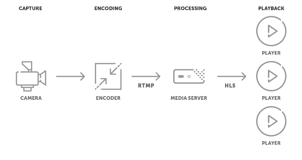
Before we look at the protocols, let’s first discuss what an entire live streaming setup looks like, from source to player. I will give a shoutout to Wowza here, a video streaming platform provider, who offer a ton of very useful blogs on video and streaming-related topics. They have drawn up a nice diagram of a simple live streaming setup:
Now, in our case we won’t be using a camera, but an application to generate the images, but the principle remains the same:
First you pass your video frames through an encoder, then you stream it to a media server of some kind, which will then deliver it to multiple players. This means that we are two different connections: from our encoder to the media server, and from the media server to the players.
The process of streaming video data to a media server is known as ‘ingesting’. On this side we need to choose an ‘ingest protocol’. This is just a point-to-point connection between your application and the media server. Wowza has an in-depth blog on streaming protocols. TL;DR: the RTMP protocol, originally developed by Macromedia for Flash video, is still by far the most popular ingest protocol. And as you see in the diagram above, they also chose RTMP as the ingest protocol here.
The job of the media server then is to scale the live stream up to multiple clients. There are two main options here. We have Apple’s HTTP Live Streaming (HLS), and we have Dynamic Adaptive Streaming over HTTP (MPEG-DASH). HLS is the most popular option, but DASH is also widely supported, and both protocols are very similar in operation.
What these protocols do, is a simple trick: your source video stream is cut up into small files, which contain a few seconds of video each (this is where our fragmented/packetized encoding with GOPs is required). The player will do a HTTP request to a playlist file, which contains a list of these files in the correct order. The player will then fetch these video fragment files, again via standard HTTP requests, and play them in the correct order, and periodically refresh the index file to get the next set of video fragments.
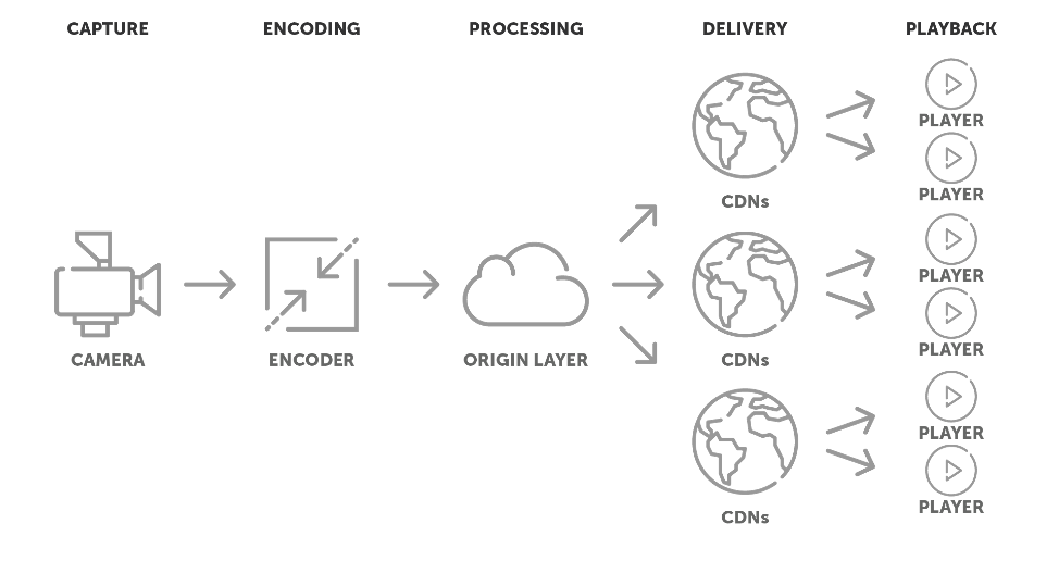
This is a typical case of divide-and-conquer: these small files can now be distributed efficiently to a number of clients. A more advanced setup will look like this:
Instead of just having a single media server, we can use so-called Content Delivery Networks (CDNs). This is the magic that allows you to scale up your livestream to millions of viewers. The files can efficiently be distributed from the ‘origin’ media server that you are ingesting to, to any number of ‘slave’ media servers. And this can be scaled up exponentially: for example, your origin server can distribute the data to say 100 slaves. Then each of these 100 slaves can feed 100 more, etc. You can add as many layers of servers as you require, and it is relatively simple to dynamically scale the capacity up or down, based on demand.
The origin layer may also perform some additional processing, such as transcoding the source data down to lower resolutions, framerates and bitrates, so that players with less bandwidth and/or less video decoding performance available can also stream the video. These would then be additional ‘variant streams’ in the HLS or DASH playlist, and players can adaptively switch to streams of different bitrates/resolutions for the best experience.
Self-hosting or using a video platform
Depending on your use-case, you may want to either host the entire platform yourself, or plug into a video platform of a third party. Either way, you will probably be ingesting via RTMP, so that is what I want to cover here. But setting up a local media server doesn’t have to be that difficult, and it makes testing easier as well, during development. So I will give some pointers here.
One simple solution is the popular web server nginx. There is an RTMP module available for nginx, which allows RTMP ingestion and output to HLS and DASH. It is not enabled by default, so if you build it from source, you need to configure it to build with RTMP. For Windows, I found this prebuilt version, which comes set up with HLS and DASH test pages and all. For my initial testing, I used this nginx setup.
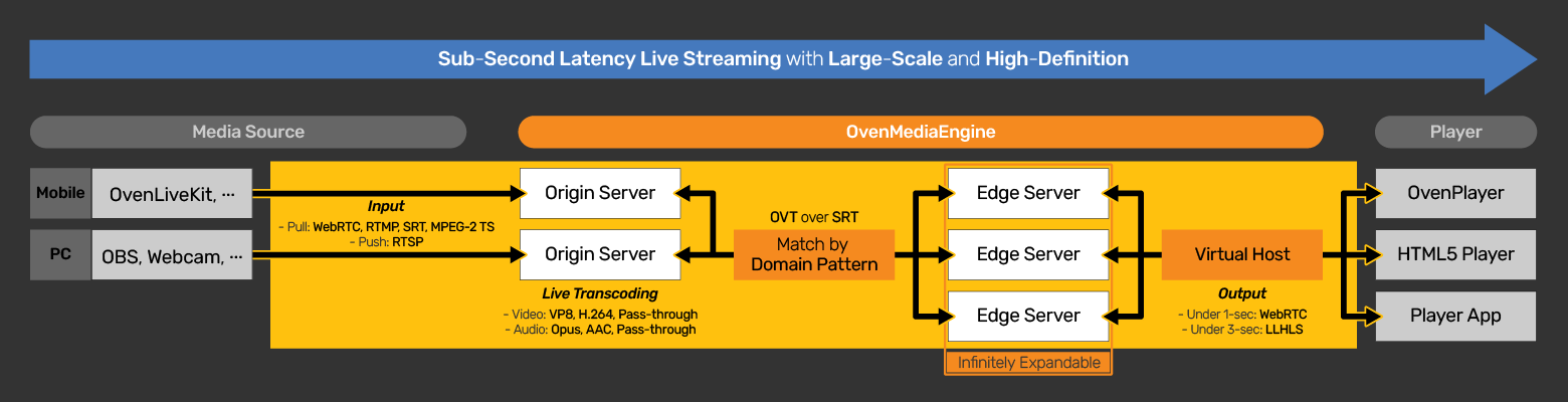
There are also various dedicated media servers available, including free/open source ones. I have used OvenMediaEngine for some more advanced testing. It is linux-only, but they provide a Docker image which can also be run under Windows. Here is the overview of the pipeline from source to player with OvenMediaEngine:
As you can see, it is similar to the earlier diagrams, but it contains some extra details, among which the various supported protocols for ingestion and delivery.
OvenMediaEngine also supports WebRTC for both ingestion and delivery to the player. WebRTC is still a relatively new and young web technology for media, but it has some interesting advantages. It is designed around the websockets available in modern browsers, and provides a JavaScript API for low-latency video transfer. It was originally designed for things like browser-based online conferencing (so peer-to-peer connections between browsers, rather than between a server and a browser), but its capabilities of sending media from one peer to another with low latency can be used for various goals, check out their samples. You can even capture streams from WebGL elements, and either stream them live to other elements, either local or remote, or record videos, and offer them for download.
Where HLS and DASH will allow you to deliver live streams and scale up to very large amounts of viewers, they tend to have a latency of 5 to 30 seconds, depending on how optimized the setup is. WebRTC can have sub-second latency. Not only does that allow a near-realtime experience, but it also means that if you have multiple players, they will play the content more in-sync, where with the older live streaming protocols you probably recognize that if you were watching the same feed as other people in a chat, some people apparently see things on the stream, and comment on them in the chat long before you do.
There are some downsides to WebRTC though. One is that there does not appear to be a fully standardized protocol for video streaming from a media server. Which means that you need a player specific to the protocol of the media server you are using. OvenMediaEngine offers its own OvenPlayer for example. Some other free opensource media servers with WebRTC support are Janus, Pion, and SRS.
Another downside is that WebRTC streaming will not scale as well as HLS or DASH will. WebRTC uses UDP rather than TCP to transfer data, which has lower latencies, but has some limitations as well. Depending on the exact implementation used, WebRTC streaming can be scaled to hundreds or thousands of users, but for really large-scale live streaming with millions of viewers, you will probably need to move to HLS or DASH. In short, WebRTC offers lower latency than HLS/DASH, but the tradeoff is in scaling.
The diagram also makes a distinction between “Origin Server” and “Edge Server”. As said before, the ‘origin’ is where ingestion happens, and any preparation of the data for streaming, such as transcoding for different resolutions/bandwidths. The edge servers are simple servers that simply distribute prepared data from the origin server to the players. A Content Delivery Network will be built up from edge servers. These edge servers can use very modest hardware, as they do not need to encode, decode or transcode any video data. They merely need to receive the fragment files from the origin server, and serve them to any connected players.
Transmuxing, not transcoding
Another relevant concept to discuss is that of ‘transmuxing’. Transcoding is probably a familiar term to most people. It involves decoding data from one format, and then re-encoding it into another format.
As mentioned above, muxing is the process of combining audio and video data into a stream. Transmuxing then is the process of extracting audio and video data from a stream, and re-encoding it into another stream.
The difference between transmuxing and transcoding then is that transmuxing does not actual decode and re-encode the video and audio data, it merely re-packages the data into a different format. This is of course a much less resource-intensive operation than a full transcode.
Now why is transmuxing relevant? As we have seen, we will require different types of protocols at different stages in the streaming pipeline. We may require one protocol for ingestion, and another protocol for delivery to players, and possibly a third protocol between origin and edge servers. So when moving from one protocol to the next, ideally we want to only perform transmuxing, rather than having to transcode the entire stream. This will keep both resource usage and latency down to the bare minimum.
So when we choose what audio and video codecs to use, we want to make sure that they are supported by all protocols along the way.
Choosing audio and video codecs
To make a long story short, as you could read in the Wowza blog on streaming protocols, the H.264 video codec is supported by every protocol out there. And as I discussed in my earlier blog on video codecs, it is a good choice, because it is reasonably modern, so you can get a good balance of quality and bandwidth, while at the same time it is supported well in hardware. So that’s an easy win.
With audio, the biggest limitation appears to be web browsers. When you want to play your video stream in a browser environment, then you are pretty much limited to AAC as a codec, since that is the only widely supported audio codec.
So we can set up a pipeline with RTMP ingestion and HLS or DASH delivery, using H.264 video encoding and AAC audio encoding, stored in a fragmented MP4 stream.
How to set it up
We need to set up our software for ingestion, in this case via RTMP. From there on, everything else can be taken care of by the media server. So, what is a good library for RTMP?
I looked around a bit for some .NET-based implementations of RTMP, but only found some vague, undocumented libraries, where it wasn’t clear what they did or didn’t implement, or how they would be used exactly.
So then I decided to look at C/C++ instead. I first looked at OBS Studio, a popular tool for live streaming, which supports streaming to a large number of platforms. It did not appear to have any clear-cut libraries for ingestion protocols. However, after some research it became clear that OBS Studio bases its RTMP implementation on FFmpeg. And FFmpeg is in fact a common tool for ad-hoc video streaming pipelines.
Now, FFmpeg is in itself not exactly a library that implements RTMP, but rather it allows you to specify various URLs and formats it can use, so you can configure it to ingest to an URL in various ways, including ones that are RTMP-compliant. This is done via the libavformat part of FFmpeg, which is where you find the muxing/demuxing functionality.
I found this example code that opens a video file and streams it via RTMP, so it can be ingested by platforms such as Vimeo. So it demuxes the input video, and remuxes it into the FLV format for RTMP compatibility. So, this is a simple example of transmuxing.
Now that we know how to ingest existing content via RTMP, the next step is to stream content that is generated in realtime by our application.
I found a slight snafu here: FFmpeg is available under both GPL and LGPL. Since my code will not be licensed under GPL, I will be using the the LGPL version. The LICENSE.md file of FFmpeg explains the differences between the two versions. One of the differences is that libx264 is under GPLv2, so it is excluded from the LGPL version. Just when we had decided that H.264 is the preferred video codec!
But, since I am on Windows anyway, and I already had an implementation of a video encoder based on Media Foundation, I figured I would be using that, as it supports H.264 out-of-the-box. But then how would I combine the two? How do I get Media Foundation to encode the video, and then get FFmpeg to ingest it? I would have to somehow connect the output of Media Foundation to the input of FFmpeg, in a way that they can communicate asynchronously. The output stream of Media Foundation will be the input stream of FFmpeg, but they have to be able to access this stream independently.
The solution I arrived at was to implement the IMFByteStream interface, where the encoder would write into a pipe. I would then do the equivalent on the FFmpeg side: create an AVIOContext via the avio_alloc_context() function, passing my own read_packet implementation that would read from this pipe. I pass no write or seek functions to the function, because we cannot support these operations on a live stream. The pipe will the take care of the asynchronous access, because it acts as a write buffer for the encoder, and it can be polled for input by the custom read_packet function.
I then had to configure Media Foundation to generate a fragmented MP4 stream so that the generated stream is in fact suitable for linear streaming. The AVIOContext allows FFmpeg to transmux the encoded video into an FLV stream and pass it to an RTMP endpoint. And there we go: we can now render frames with our application, encode them to a H.264 stream in realtime, and then ingest it to live streaming platform that supports RTMP.
I would like to give a heads-up about the new PC emulator on the block. It is called “MartyPC”, which indeed is a reference to Marty McFly from the Back To The Future movies. And indeed, that is a tribute to our 8088 MPH PC demo, which had various references to these movies.
And yes, that means that this PC emulator intends to be cycle-exact, in order to run 8088 MPH. So here is a video demonstrating it running Area 5150:
Because, long story short: The emulator started development before Area 5150 was released, but as it turns out, Area 5150 was easier to render correctly, as it doesn’t require emulation of the NTSC composite video signal. But 8088 MPH does run in the emulator as well, as developer GloriousCow assures us. He just wants to put a bit more work into the video signal to get more accurate colours, before releasing a video capture of that demo.
Speaking of video, note that MartyPC correctly renders the ENTIRE display area, including overscan, which means we get proper borders and overscanned effects, as used in Area 5150.
So wait, didn’t we already have an emulator that runs 8088 MPH? No, I said we had an emulator that *doesn’t break* when running 8088 MPH. It was close, but it was not cycle-exact, so it didn’t look exactly the same as on real hardware. It would speed up or slow down in various parts.
Not this emulator. MartyPC really *is* cycle-exact. And it is open source, available on Github. And as you can see, it is written in Rust. A somewhat unusual choice for emulators, as they are mostly written in C or C++. But Rust is an interesting and very new and modern language, and it is very suitable for this sort of low-level work.
What’s also cool is that GloriousCow is documenting his work on his blog. He has only just started blogging, so at the time of writing there are only two technical articles (one on DMA, and one on CGA waitstates). But they are very detailed, and very readable as well, with diagrams, oscilloscope signal views and whatnot, so this looks very promising indeed!
All in all, this is finally a PC emulator that TRULY tries to do exactly what the hardware does. Which has been a pet peeve of mine for years, given that emulators for most other platforms have been designed this way.
For that, we can check the IBM PCjr Technical Reference, page 2-107 onward. Apparently a cartridge merely contains a ROM, which needs to have a certain header in order to be detected. It starts with the bytes 55h, AAh, and then a length-field (in blocks of 512 bytes). Then 3 bytes where you can store a jump to your initialization routine entry-point. The byte after that, at offset 6, will indicate what type of cartridge it is.
Three types of cartridge are supported:
“Initial Program Loadable” (IPL): The cartridge will register an INT 18h handler for itself at initialization. INT 18h will be called after the BIOS POST is done, and no bootable device was found. This is the mechanism by which BASIC is normally started on an IBM PC or PCjr. BASIC is then the ‘initial program’ that is loaded. When the type-byte at offset 6 is set to 0, the cartridge is expected to be an IPL-type.
DOS Command Extensions: From offset 6 onwards, a list of commands is stored: first a length-byte indicating the length of the command. Then the ASCII-string of the command itself, followed by a (word) offset to the code that implements the command, according to the manual. However, that seems to be an error. Instead, DOS will jump directly to the position directly after the command-string. You have 3 bytes to put a jump to the actual code, similar to the main initialization entry-point (DOS creates a process for you, so you can just use ah=4Ch to exit back to DOS from your command). The list of commands is terminated by an entry with a length of 0.
BASIC cartridges: Instead of the 3-byte jump at offset 3, you have the sequence: CBh, 55h, AAh. The type-byte at offset 6 will be set to 0. Then at offset 7, there will be a byte that is either FEh for a protected BASIC program, or FFh for unprotected.
After this initial header, the code (either x86 machine code or BASIC) will be stored, and at the end of the image, there will be two bytes that contain a 16-bit CRC code. We will get back to that later.
But first… did you see what they did there? With the 3 types? They tricked us! Because if you consider a DOS command image with no commands, then technically it is the same as an IPL-type. What you do in the initialization code is pure semantics. And the CBh byte for the BASIC cartridge is actually a RETF instruction. So that is technically an empty initialization function. Apparently the BIOS can still call into it, it will just return immediately. The 55h and AAh bytes are then additional bytes that BASIC can check for at a later point. Likewise it seems that the DOS commands are actually scanned by DOS at a later part in the boot sequence, not during BIOS initialization. So what this appears to boil down to is that the BIOS merely checks for valid ROMs by scanning for the 55h AAh marker, then checking the length and verifying the CRC value, and if that checks out, it will do a far-call into offset 3 to call the initialization routine of the ROM.
But we can trick them as well, can’t we? Yes, it would seem that although the jump at offset 3 should technically be jumping into an initialization function, and then RETF back to the BIOS initialization, in practice various cartridges actually jump directly into the program code, and just never return to the BIOS at all. This fundamentally changes how the cartridge works: If you just use the initialization routine to install an INT 18h handler, then the cartridge code will only be executed when no bootable device is found (so only when you have not inserted a bootable floppy, and you have no other boot device, such as a HDD installed). If you start your application code directly from the init function, then it will execute regardless of whether other boot devices are available.
If you compare this cartridge system with the BIOS extension system of the regular IBM PC and compatibles, you’ll find that it works in basically the same way. You can find it in the IBM PC Technical Reference, page 5-13 onward. That is, the PC BIOS does not appear to support DOS command extensions or BASIC extensions via ROM, but an IPL-type ROM for PCjr is very similar to a PC BIOS extension. The initial 55h, AAh bytes and the length-value are stored in the same way. And in both cases the BIOS will also do a far-call to offset 3. The PCjr simply extended this mechanism by jumping over the optional DOS commands that can be stored, starting at offset 6.
Also, where the PCjr uses a CRC16 to verify the ROM, the PC BIOS uses a simple checksum (just adding all bytes together, modulo 100h). But the idea is the same: after processing all bytes in the ROM, the CRC16 or checksum should be 0, so you should add a value at the end of your ROM to make sure it gets to 0. That will make it somewhat difficult to make a single ROM that works on both types of machines (it would need to pass both the CRC16 and the checksum-test), but you can trivially make both a PC and a PCjr version out of the same codebase, by only adjusting the CRC/checksum-value for the specific target before writing it to a ROM.
The address range of the ROMs is also different: the PC BIOS extensions use the segment range C000h-F400h, where the PCjr cartridge uses segment range D000h-F000h (allowing to add up to 128k of ROM space via two cartridges). In both cases, the ROM area is scanned at an interval of 2k blocks. So a new ROM image (indicated by the 55h AAh marker) can occur at every 2k boundary. The PCjr simply treats ROMs at D000h and above as cartridge ROMs (and as such expects CRC16), where the rest are assumed to be standard BIOS extensions (with a checksum).
So in theory you can create a ROM containing an application for a regular IBM PC as well, and stick it onto an ISA card, as a makeshift ‘cartridge’. In practice it’s just less convenient as you cannot easily insert and remove it. That might explain why the support for DOS command or BASIC expansion ROMs was never added to regular PCs, and as such, remains a PCjr-exclusive.
However, the cartridge port on the PCjr is basically just a cut-down ISA slot. In theory you could create an ISA card with a PCjr-like cartridge slot in the bracket at the back, so that you can insert cartridges with ROMs that way. And once you can easily insert and remove ROMs like that, it makes sense to create ROMs that contain games or other software.
Why cartridges/ROMs?
Is there a point to using cartridges/ROMs, you may ask? Can’t you just load your software from a floppy or harddisk? Well yes, there is. Roughly there are two advantages to storing software in ROM:
The ROM is mapped into a separate part of the address space, so your code and data can be accessed directly from the ROM, leaving your RAM free for other things.
Unlike the dynamic RAM in your machine, the ROM does not need to be refreshed. As such, when reading from ROM, you do not incur any waitstates. This makes ROM slightly faster than RAM.
For a regular PC this is not such a big issue, as they generally have lots of RAM anyway, and a regular PC refreshes memory only once every 18 IO cycles (roughly every 15 microseconds).
For a PCjr however, things are different. A standard PCjr has only 64k or 128k of memory, and this is shared with the video circuit. So it reserves 16k to 32k of video memory from this pool. The 64k models were sold without a floppy drive, as DOS would not be much use in the remaining 48k of memory. Even 128k is still quite cramped for DOS. So if you could store your application in ROM, you can make more of the system RAM.
And PCjr shares its main memory between the CPU and the video chip. This means you don’t get a memory refresh cycle once every 18 IO cycles. Instead, the video circuit will access memory once every 4 IO cycles, generating a wait state that blocks the CPU from accessing memory. Effectively this makes the CPU run code much slower from system RAM than from ROM or expansion RAM. Putting code and data in a ROM cartridge will fix this performance disadvantage of the PCjr, making it run as fast as a regular PC (or actually slightly faster).
Lotus 1-2-3 was released on two cartridges for the PCjr at the time, as the application itself was already 128k in size. It was still a DOS application, the cartridge made use of the DOS command extension mechanism to register ‘123’ as a command, so it would start from the cartridge when you entered ‘123’ at the DOS prompt. That was a clever way to make the most of the PCjr. It ran from DOS, so you would have access to floppy storage without any issues. It saved precious system memory by storing the application in ROM. And the ROM also made the code run faster than if it were a regular DOS application running from RAM.
So let’s see what it takes to make our own cartridge.
The CRC check
Let’s look closer at how the CRC check works. We are going to need it in order to pass the validation check in the BIOS, so it will actually run our code from the ROM.
On page 2-109, the Technical Reference points to the ‘crc_check’ routine in the BIOS listing, to see how this works. We can find this CRC routine on page A-106:
So the CRC check basically scans the entire ROM image (including all headers), and the check passes if the resulting CRC value is 0.
On page 2-108, the manual says that you should put ‘CRC Bytes’ at the Last 2 Addresses’ of your ROM image. What they mean to say is that the CRC should yield 0. But the CRC is just a polynomial calculated over the ROM contents, so it can be anything, depending on the contents. In order to get it to 0, you need to add extra ‘dummy bytes’ to get the polynomial to reach 0 at the end. And since this is a 16-bit CRC, two bytes are enough to compensate.
But if you study the code, you see that it simply calculates the CRC over the entire area, and doesn’t specifically treat the last two bytes as something special. This means that theoretically you can place them anywhere in your image. In fact, in the rare case that the CRC already reaches 0 without adding extra bytes, you can just leave them out altogether.
However, in practice, it is easiest to place them at the end. Namely, how do you generate these two bytes? Well, one way is to just bruteforce all options (there are only 65536 possibilities), until you find one. But if you have to calculate the CRC over the entire ROM every time, this will be relatively inefficient. CRC is an incremental algorithm however. That is, you start out with an initial value (which by default is FFFFh as you can see in the code), and then add on to that.
So if you want to bruteforce the last two bytes of a ROM image of N bytes, you simply calculate the CRC up to N-2 bytes first. Then you use this CRC as the initial value, and calculate a CRC for the last two bytes. So you only have to calculate up to 65536 CRCs of 2 bytes in order to find the right combination. Even an 8088 at 4.77 MHz can do that almost instantly.
Writing the code
It’s somewhat tricky to write actual ROM code, because the usual programming environments are aimed at DOS, and as such want to generate either a .COM or a .EXE file. Generating a valid ROM image is not directly possible with most programming environments. A .COM file is pretty close to a raw binary image though: it is a single segment of up to 64k in size, containing both code and data. Obviously you have to avoid any dependencies on DOS in the .COM file, so you probably need to disable any runtime libraries. In which case the main difference with a raw binary is that a .COM file starts at offset 100h.
This is another DOS-dependency, as DOS creates a Program Segment Prefix (PSP) block for every process that it starts. This block is 256 bytes long, and the .COM file is loaded directly after it, in the same segment. DOS will then call the code at offset 100h as your entry point.
In a cartridge we do not have a PSP, but we do have a header, with a jump into the actual code. This header is much smaller than 256 bytes. So we could create a cartridge header with a jump to 100h, then pad up to offset 100h, and then append the .COM file there.
However, I chose to use MASM, and in that case you specifically have to place a ‘org 100h’ directive to make the code start at offset 100h. If you omit that directive, it will start the code (or data) at offset 0. This means I can actually place the header inside my assembly code, and place my code and data directly after the cartridge header. I created a template like so:
.Model Tiny

.code
; Cartridge header
marker dw 0AA55h
len db 0
jmp InitROM
; List of DOS commands
org 6
db 0

; Start of ROM data

InitROM PROC
...
retf
InitROM ENDP

...

END
The generated .COM file will then start with the header, and the code will correctly assume that the image is loaded at offset 0 in the segment, not offset 100h. There are just three problems left:
The length-field is left at 0, because it should be specified in blocks of 512 bytes. While it is possible to do simple addition and subtraction with labels in MASM to get the size of a block of code or data, it is not possible to divide the size by 512. So we cannot let the assembler generate the correct length in the image automatically.
The image size needs to be aligned to blocks of 512 bytes. The assembler can only do alignment up to 256 bytes (the size of a ‘page’).
The image needs to generate a CRC value of 0, which as mentioned above, will require adding additional bytes to adjust the CRC.
I have created a simple tool for this, based on the actual BIOS code. It checks if the length-field matches with the actual size of the binary. If there is a match, it assumes the image is already prepared for a cartridge, and it will calculate the CRC for the image, and report whether it is 0 or not.
If the size is a mismatch, it will assume the image needs to be prepared. It will first add two bytes to the size, to make room for the CRC adjustment. Then it will align the size up to the next 512-byte boundary, and write the size into the header. Then it will calculate the CRC for the entire image, save for the last two bytes. The final step is to bruteforce the last two bytes to find a value that gives a CRC result of 0. These are then written to the image, and the result should be a valid cartridge image.
I will probably put this tool in the DOS SDK when it has matured a bit. If you are curious, other people have also created cartridges, and released tools, for example, this entry on Hackaday by SHAOS.
For completeness, this more elaborate template demonstrates an initialization function, which registers an int 18h handler, and implements two DOS commands:
.8086
.Model Tiny

; Macro to make sure the jump to the command always takes 3 bytes
CARTPROC MACRO target
	LOCAL start

	start EQU $

	jmp target	; This must be a 3-byte field, so a relative jump with 16-bit offset, or else pad with a nop before the next command
	org (start+3)
ENDM

; Macro to add a DOS Command to the header
DOSCOMMAND MACRO cmd, target
	LOCAL str

	db SIZEOF str	; Length of command string
	str db cmd	; Command must be uppercase

	CARTPROC target	; Add 3-byte jump code to command proc
ENDM

.code
; Cartridge Header
marker dw 0AA55h
len db 0
jmp InitROM
org 6

; DOS Commands
DOSCOMMAND "TEST1", test1
DOSCOMMAND "TEST2", test2

; End DOS Commands
db 0

; Zero-terminated string in DS:SI
Print PROC
	; Get current video mode, so current page is set in BH
	mov ah, 0Fh
	int 10h

	lodsb
	test al, al
	je done

outputString:
		; Output char to TTY
		mov ah, 0Eh
		int 10h

		lodsb
		test al, al
		jne outputString
done:
	ret
Print ENDP

; Start of ROM data
InitROM PROC
	mov si, offset initString
	call Print

	; Set INT18h handler
	pushf
	cli

	push ds
	xor ax, ax
	mov ds, ax

	mov ds:[18h*4 + 0], offset EntryPoint
	mov ds:[18h*4 + 2], cs

	pop ds
	popf

	retf
InitROM ENDP

EntryPoint PROC
	sti

	push cs
	pop ds

	mov si, offset entryString
	call Print

	iret
EntryPoint ENDP

initString db "Cartridge Initialization",0
entryString db "Cartridge EntryPoint",0

test1str db "test1",0
test2str db "test2",0

test1 PROC
	push ds
	push cs
	pop ds

	mov si, offset test1str
	call Print

	pop ds

	mov ax, 4C00h
	int 21h
test1 ENDP

test2 PROC
	push ds
	push cs
	pop ds

	mov si, offset test2str
	call Print

	pop ds

	mov ax, 4C00h
	int 21h
test2 ENDP

.data

END
That gives you all the possible functionality, aside from BASIC stuff. You could combine everything in a single cartridge as this template demonstrates, but the idea is to just show the different techniques, so you can pick and choose. If you just want a DOS cartridge, you don’t need the initialization and int 18h handlers. Just a retf at initialization is good enough.
And the int 18h setup is only for when you want the cartridge to start only when no boot device is found. So you can control whether or not to run the cartridge by inserting a bootable floppy. If you want the cartridge to always run when inserted, just put your code directly in the inititalization.
Running the cartridge code
Now that we know how to create a cartridge image, how do we actually run and test it? The easiest way to do a quick test is to use an emulator. A file format for PCjr cartridges exists, originally developed for the Tand-Em emulator (which, as the name implies, was originally a Tandy 1000 emulator, but the PCjr is of course a close relative). A utility by the name of JRipCart was developed to extract PCjr cartridges to files with the extension .JRC, for use in emulators. The JRC format is very simple. It’s just a header of 512 bytes in size, with some metadata about the ROM, which is prepended to a raw cartridge image. You can easily make the header yourself, and then use the copy-command to append the two files into a new .JRC file:
copy /b HEADER.JRC+CARTRIDGE.BIN CARTRIDGE.JRC
A popular PCjr emulator with support for .JRC is DOSBox. You can load a .JRC file via the ‘BOOT’ command when you are using the PCjr machine configuration, similar to how you’d boot a floppy image. Note that DOSBox support is very limited, and the current release at time of writing, .074-3, does not actually verify the length field or the CRC, so it does not tell you whether or not your cartridge ROM is fully valid. It merely loads the ROM and executes the code from offset 3.
But of course we would also want to run it on actual hardware. There are various ways to do that. You can go the ‘classic’ way of creating an actual PCB with ROMs on it. You can find the schematics online from various projects, including one from SHAOS, or from Raphnet. The SHAOS-design is true to the original PCjr cartridges, and uses 32k EPROMs. So you need two 32k EPROMs for a 64k cartridge. Raphnet uses a design based around a more modern EPROM type which is available in 64k, so a single EPROM is enough (although it requires a 74LS08 IC for some glue-logic).
Speaking of Raphnet, he has also developed an interesting PCjr cartridge, which allows you to use an SD-card as a harddisk. That is especially interesting since the cartridge port is a read-only interface. So the design uses a clever hack to allow writing to the device as well.
However, this design currently does not allow you to store cartridge images on the SD-card, and load them as ROMs, as far as I understand. There is another device available, which can do exactly that, the BackBit Pro cartridge:
I don’t currently have the tools to (re)program EPROMs.
Using an SD-card is more convenient than having to reprogram EPROMs and putting them on a PCB everytime during development.
I suppose once you’ve developed and tested your cartridge image, you can always have a ‘real’ EPROM cartridge made from it later.
The BackBit Pro cartridge is a very interesting device, in that it is a ‘universal’ cartridge, that you plug into a suitable adapter for your target system. There is quite a selection of adapters available, and last year, a PCjr adapter has been added:
It works in a way similar to other devices that simulate cartridges, floppy drives and such via SD-cards, USB drives and whatnot: When you boot up the system (or press the reset button), a menu pops up, which allows you to browse the SD-card and select a ROM file. The system then reboots and runs the cartridge.
The BackBit Pro has a few other tricks up its sleeve. Aside from emulating cartridges, it can also be used to load alternative BIOSes (these were a thing on the PCjr, for example, to make it appear like a regular PC for better compatibility, or to skip the REALLY slow memory test when you have a large memory expansion). And it can load .COM files or floppy images directly (great for booter games).
The current version only seems to support raw cartridge images, which have to have the .BIN extension. It does not appear to support .JRC files yet. But that’s not a big deal, as it’s trivial to convert a .JRC to a raw image: just cut off the first 512 bytes.
I also had some issues with my jr-IDE installed: the BackBit Pro selection screen would not start. You would see it change the border colour to its characteristic pink colour, but then the system froze. Other than that I didn’t encounter any problems, so I can certainly recommend the BackBit Pro for cartridge development, or just as a nice tool for running software on the PCjr.
Update (5-6-2023): The BackBit Pro has received a firmware update (2.1.2), which solves the issue with the jr-IDE. Apparently the issue was that the jr-IDE switched to 80-column mode, which also enables a different page of video memory. So the BackBit Pro was actually working, it was just updating a part of VRAM that was not visible at the time. It now switches back to 40-column mode and a known page of display, which fixes the issue. I think in general it’s a good idea not to make assumptions about what mode and display page you’re in, when writing BIOS or cartridge ROMs. I have found some issues with using the BIOS int 10h TTY output from a cartridge as well.
The firmware also adds support for .JRC files, so you don’t need to convert them before copying them to your SD-card. Excellent work!
Anyway, hope this has been a helpful primer into the world of PC/PCjr cartridges and BIOS extension ROMs.
A few months ago, I discussed downgrading a modern codebase to .NET 4 and Windows XP. I managed to get the code working to the point that all functionality worked, aside from web views, given that browsers no longer support XP or Vista. The .NET 4/XP version of the application makes use of a DirectX 9 renderer and DirectShow or VLC for video playback. DirectX 9 you say? Well, I suppose I have to be more specific. So far we have only looked at the software side of things: which components, frameworks, libraries, APIs etc. are supported on Windows XP? But we worked under the assumption that the hardware had the same capabilities as the hardware that ran newer versions of Windows. Under certain circumstances, your software will also be limited by the capabilities of your hardware. This is especially true for DirectX, as it is a low-level hardware abstraction layer: it abstracts the hardware you have, but as a rule it does not emulate the hardware you don’t have.
DirectX 9, the Swiss Army Knife of graphics APIs
As said, this codebase started life around 2008, at which time shader hardware was standard, even with low-end integrated GPUs. The Aero desktop required a minimum of a DirectX 9 GPU capable of Shader Model 2.0. The codebase made use of shaders through the Direct3D Effect Framework. DirectX 9 is an interesting API as it covers a lot of ground in terms of supported hardware. While at the high-end, it supports Shader Model 3.0, with floating point pixelshading, branching and whatnot, it also supports the first generation SM1.x hardware, and even the pre-shader hardware that was designed for DirectX 7 and below, where we had a fixed function pipeline. So DirectX 9 allows you to go all the way from relatively early 3D accelerators, such as an nVidia TNT or GeForce, or the original ATi Radeon, all the way up to floating-point shader cards. Crysis is a good example of what you can do with DirectX 9 when pushed to the extreme. The original Crysis had both a DirectX 9 and a DirectX 10 backend. While the DirectX 10 rendering quality was absolutely groundbreaking at the time, its DirectX 9 mode is not even that much of a step backwards visually, and it will run on Windows XP systems as well. Earlier games, like Far Cry and Half Life 2, would use DirectX 9 to support a wide range of hardware from fixed function all the way up to SM3.0.
But can our application also support this wide range of hardware? Now, as you may recall from some of my earlier exploits with old GPUs, recent DirectX SDKs include a compiler that will output only SM2.0 code or higher, even if the source code is written for a lower shader version. This also applies to Effects. As far as I can tell, our software has always used this modern compiler, or at the least, all shaders assumed SM2.0 or higher. You need to use an older compiler if you want to use Effects on actual SM1.x or fixed function hardware, otherwise the compiler will silently promote effects to SM2.0, and will only work on SM2.0+ hardware.
We build and distribute our application with pre-compiled shaders. We use the fxc.exe shader compiler for that. I had already created some scripts that compile a set of DX9 and a set of DX11 shaders separately, as the two APIs cannot share the same shaders. So I introduced a third set here, which I called ‘dx9_legacy’. Then I grabbed the old fxc.exe compiler from the June 2010 DirectX SDK, which seems to be the last to support the older shader models and fixed function. I renamed the old fxc.exe to fxc_legacy.exe and added it to the build with a script to compile a new set of shaders from a dx9_legacy source folder and output to a dx9_legacy folder.
From there, I had to modify the application to support these alternative Effect files. That was relatively simple. Like before, I had to add the D3DXSHADER_USE_LEGACY_D3DX9_31_DLL flag when loading these legacy Effects. Or in this case, it’s actually the SharpDX equivalent: ShaderFlags.UseLegacyD3DX9_31Dll.
And I had to select the proper set of Effects. That is quite simple, really: if the hardware supports SM2.0 or higher, then you don’t need the legacy shaders, else you do. It gets somewhat more complicated if you want to support every single version of hardware (fixed function, ps1.1, ps1.3 and ps1.4). Then you may want to have a separate set for each variation. But at least in theory, I can run any kind of code on any kind of hardware supported by DirectX 9 now, as the legacy compiler can compile Effects for all possible hardware (it can also do SM2.0+, although the newer compiler will likely generate more efficient code).
More specifically, I only had to check if Pixel Shader 2 or higher was supported. Namely, first of all, the new shader compiler still supports Vertex Shader 1.1. Only pixel shaders are promoted to ps2.0. And secondly, there is the option for software vertex processing, where DirectX 9 can emulate up to vs3.0 for you. In my case, the vertex shading is relatively simple, and meshes have low polycount, so software processing is not an issue. Which is good, because that means I do not have to build a fixed function vertex processing pipeline next to the current shader-based one. All I have to do is rewrite the pixel shader code to fixed function routines, and the code should run correctly.
Or actually, there was a slight snafu. Apparently someone once built a check into the code, to see if the device supports SM2.0 at a minimum. It generates an exception if it does not, which terminates the application. So I decided to modify the check and merely log a warning if this happens. It’s purely theoretical at this point anyway. Hardware that does not support SM2.0+ has been EOL for years now, so it is unlikely that anyone will even try to run the code on such hardware, let alone that they expect it to work. But with our legacy compiler we now actually CAN make it work on that hardware.
A willing test subject
I have just the machine to test this code on. A Packard Bell iGo laptop from 2003 (which appears to be a rebadged NEC Versa M300):
It is powered by a single-core Celeron Northwood (Pentium 4 derivative) at 1.6 GHz. The video chip is an ATi Radeon 340M IGP. The display panel has a resolution of 1024×768. It originally came with 256MB of memory and a 20 GB HDD. These have been upgraded to 512MB (the maximum supported by the chipset) and a 60 GB HDD. It came with Windows XP Home preinstalled, and that installation is still on there.
The Radeon 340M IGP is an interesting contraption. It reports that it supports Vertex Shader 1.1 in hardware, but it is likely that this is emulated on the CPU in the driver. The pixel pipeline is pure DirectX 7-level: it is taken from the original Radeon, codename R100. It supports three textures per pass, and supports a large variety of texture operations. This is exactly what we like to test: Effects with a simple vertex shader, and fixed function pixel processing.
So I started by converting a single Effect to vs1.1 and fixed function. I chose the Effect that is most commonly used, for rendering text and images, among others. This will be my proof-of-concept. I first developed it on a modern Windows 11 machine, where it appeared to render more or less correctly. That is, the alphachannel wasn’t working as it is supposed to, but text and images basically appeared at the correct place on screen, and with the correct colours, aside from where they should have been alphablended.
Well, good enough for a proof-of-concept, so I decided to move over to the old laptop. Initially, it opened the application window, which is good. But then it didn’t display anything at all, which is bad. So I looked in the log files, and found that there were some null pointer exceptions regarding font access.
Interesting, as the application had been made robust against missing fonts in general. But as I looked closer, this was for the initialization of some debug overlays, where there was some special-case code. We use the Consolas font for certain debug overlays, as it is a common monospace font. However, apparently it is not THAT common. I hadn’t run into this problem on my other Windows XP machines. But as it appears, the Consolas font was not shipped with Windows XP. It could be installed by various other software though, such as recent Office applications. That might explain why the font was available on my other Windows XP machines, but not on this one. So as the application initialized the overlays on startup, it tripped over the missing font, and could not recover.
I added the font to the system, and tried again, and indeed: the application now worked, and rendered exactly the same as on the modern system. So the proof-of-concept works. For completeness I also added some checks to the code, so it will not crash on missing fonts in the future.
Success
This proof-of-concept shows that everything is in place, at least from a technical point-of-view, for the support of non-shader hardware. We can compile Effect files for non-SM2.0 hardware, and load them from our application. We can create a DirectX 9 device on the old hardware, and detect when to use the fallback for the legacy compiler and alternative legacy Effect files.
The only thing that remains is to actually write these Effect files. I will probably not convert all of them, and certain ones will not convert to fixed function anyway, as they are too advanced. But I will at least see if I can fix the alphablending and add support for video playback, and perhaps some other low-hanging fruit, so that basic stuff will display correctly.
It’s interesting how far you can stretch a single codebase, in terms of development tools, APIs, hardware and OS support. On this old laptop, the code can work fine, in theory. You now run into practical problems… For example, yes it supports video playback, with a wide range of formats. But it has very limited capabilities for hardware acceleration, especially for more modern codecs. Also, we are now back to a screen with 4:3 aspect ratio, where our content has been aimed at 16:9 for many years, and more specifically 1080p, which is far higher resolution than this system can handle. Also, we normally have 2GB of memory as the absolute minimum. This system only has 512MB, and that is shared with the IGP as well. You can configure how much of it to reserve for the IGP. By default it is set to 32MB, so you only have 480MB left for Windows and your application. That puts some limits on the fonts, images and videos you want to use, as you may run out of memory simply because your source material is too big.
But, at least in theory, the code can not only run on Windows XP, but it can actually be made to run on the hardware of that era. With the right combination of content and Effect files, you can use this laptop from 2003. So where I normally use a 1080p30 test video with H.264 encoding, in this case I had to transcode it down to 720×480 to get it playing properly. H.264 does not seem to bother the system that much, once you install something like the LAV Filters to get support in DirectShow (you need an older version that still works on XP). But decoding frames of 1920×1080 seems to push the system beyond its limits. It does not appear to have enough memory bandwidth and capacity for such resolutions. Back in 2003, HD wasn’t really a thing yet. You were happy to play your SD DVDs in fullscreen.
As I converted a few Effects down to fixed function, I concluded that it is highly unlikely that this code had ever been used on non-shader hardware before. Certain implementation details were not compatible with fixed function. For example, certain constants, such as solid colour or opacity (alphachannel) values were multiplied in the pixel shader, while the vertex shader merely copied the vertex colour. With fixed function, there are a few constant registers that you could use, but that would require setting these registers specifically in your Effect, instead of setting shader constants. But since these are constants, it makes much more sense to calculate them in the vertex shader, and just output a single diffuse colour, which can be used directly in the fixed function pipeline. It is simpler and more efficient.
In general there’s a simple rule to follow… In order from least to most instances per scene, we have:
The world
Objects
Meshes
Vertices
Pixels
So, you want to process everything at the highest possible stage where it is invariant. For example, the lights and camera are generally static for everything in the world for an entire frame (they are ‘global’). So you only need to set them up once. You don’t recalculate them for every object, mesh or vertex, let alone every pixel. So in general you only want to calculate things in shaders that you cannot precalc on the CPU and pass to the shaders as constants efficiently. And you don’t want to calculate things in a pixel shader that you can calculate in a vertex shader. After all, there are normally far fewer vertices in your scene than there are pixels, so the vertex shader will be executed a lot less often than the pixel shader.
Another interesting detail is that the fonts were stored in an 8-bit format. This was effectively an alphablend value. The text colour was set to an Effect constant, so that a single font could be rendered in any colour. However, the format chosen for the texture was L8 (8-bit luminance). In the pixel shader, this value was read, and then copied to the A component, while the RGB components were set to the constant colour. I couldn’t find a way to make this work with fixed function. The fixed function pipeline treats colour and alpha operations as two separate/parallel pipelines. For each stage you can calculate RGB separately from A. However, most operations will not allow you to move data from RGB to A or vice versa. And when you read an L8 texture, the value is copied to RGB, where A will always be 1, as the texture does not contain alpha information.
So instead, the font should be using an A8 format (8-bit alpha) instead. Then A will contain the value, and RGB will read as 1, because the texture does not contain colour information. That is how the shader should also have been designed, semantically. It should have read the A-component of the texture into the A-value of the output pixel, rather than reading the RGB components into the A-value.
So this once again shows that older systems/environments have limitations that can give valuable insights in the weaknesses of your codebase, and can make your codebase more efficient and more robust in ways that you might not normally explore.
I have decided to once again port back the small fixes and modifications to the current codebase. This way I can develop the legacy Effects on the current build of our software, and do not need to rely specifically on the .NET 4 version. I have decided not to actually put the legacy Effect source code and compiler into the main codebase though. Otherwise the legacy shader set would end up in production code. However, the code knows of this set, so if you manually copy it to the correct place on disk, it will automatically make use of it.